Part 1: 1.2. Interior Space Architecture in aPBLandscape for Organismic aFootball
Space species in the Organismic Football Playground
- 2. Interior Space Architecture in aPBLandscape for Organismic aFootball
- 2.1. Affordances, Landscape Fitness and aFICS Literacy
- 2.2. Graph Model of the Interior of the Patched Landscape
- 2.3. Affordance of Organismic aFootball: Core-Convex_Hull Subspaces Control
- 2.4. Network Properties of Space Architecture of aPLandscape
- Table 1.2.1. Number of Paths of i-adjacency length in the interior of aPLandscape
- Table 1.2.2. i-adjacency length of all possible single source patch-to-patch interactions in the interior of aPLandscape
- Table 1.2.3. Set of Network Properties of PL Graph Model of the Interior of aPLandscape
- Table 1.2.4. Betweenness Centrality Contribution of each Patch
- 2.4.1 Organization of Space in Meso Subspaces Sets
- 2.4.2. Value of Patch Subspaces Control
- 2.4.3. Hierarchy of Species of Subspaces in the aPLandscape
” …after all, on the pitch what we see are plays, not data” - Clement Lengled
"There is no exterior, just interior in the closed aFICS Football Universe and it is full of affordances” - aF Vision
"The main affordance of interior space architecture invites and constrain to play in an organismic aFootball style” - aF Vision
#collapse_hide
from __future__ import print_function

# Base Computational Geometry of the Environment in Python
#Set of Fundamental packages
# scientific packages
import numpy as np
import scipy
import scipy.spatial

# data science packages
import pandas as pd

# visualization packages
import matplotlib
import matplotlib.pyplot as plt
import matplotlib.gridspec as gridspec

# animation packages
import ipywidgets as widgets
import moviepy as mpy


from IPython.core.interactiveshell import InteractiveShell
from IPython.display import display
from IPython.display import display_html, display_jpeg, display_png, display_json, display_latex, display_pretty, display_svg
from IPython.display import Image
from matplotlib.patches import Polygon,Arc,Ellipse
from datetime import datetime
from ipywidgets import interact, interactive, fixed, interact_manual

from moviepy.editor import VideoClip
from moviepy.video.io.bindings import mplfig_to_npimage

                                    #from matplotlib import colors
%matplotlib inline
%matplotlib ipympl
%load_ext autoreload
%autoreload 2

%config InlineBackend.figure_format = 'retina'
plt.style.use('fivethirtyeight')
#collapse_hide
import networkx as nx

from nxviz import CircosPlot, ArcPlot, MatrixPlot #for network vizualization
from datetime import datetime
from collections import Counter
#import numpy as np

import warnings
#from custom import load_data as cf
#warning.filterwarnings('ignore')

#%matplotlib inline
#import matplotlib
#import matplotlib.pyplot as plt
#%load_ext autoreload
#%autoreload 2
%config InlineBackend.figure_format = 'retina'
plt.style.use('fivethirtyeight')
Gon, playing alone, is learning to explore and exploit the aPBLandscape. He is instructed to observe and perceive the environment in behavioral terms or as processes. The set of things (goals, perimeter, patch-zones, the ball) in the playground, provides opportunities for and constrains his agency to move himself out-ball control or on-ball control in the next direction or next play, or have cognition of the affordances in order to answer the great question:
What is like to play football?
That in Gon's circunstances, only depends on the channeling that all 'actual affordances' perceived by him constrain his 'autonomy' in the context of his own aFICS skills and his football action capabilities.
Affordances constitute a fluid process in the coupled dynamical system Gon-aPBLandscape, scaled to his action capabilities (strength, speed, reaction times, height, weight, body dimensions) and, affordances are perceived by Gon as he learn to establish a Gon-aPBLandscape fit.
Academia Emeritense knows that its first cognitive task in Gon’s aFICS footbal education is help him to acquire the idea of perceive the patched landscape, and later the pitch, in relation to constrain its functionality as a footballer. Its meaning is rooted in the affordances that provide insights in what Gon learns and how he accomplished the motor task with open inteligence that guides the 'reduced' decision making process of how and when to act1.
Gon and Acadenia Emeritense know that learning a skill must be understood as the emergence of an adaptive, functional dynamic and constrained relation between he and his football environment fitness. This fit is influenced by a set of constrains, always present, due to
- His individual biophysical, emotional, mental and psycological constrains and,
- Environmental physical, perimeter, patch-inherents constrains, and most important
- its set of affordances offered to him in any event
All of them must be used and exploited by Gon as opportunities for his agency in the aPBLandscape and his actions will be observed by the head coach HC as a metric of his basic aFICS literacy.
In this perspective, Gon involves understanding of his whole body -embodied- with affordances offered by the -embedded- aPBLandscape will determine his agency or task performance in the ground play.
aFICS literacy is the metric used during his aFICS synergon development process until he left Academia Emeritense. Literacy must be understood by our talents as ‘being educated’ in our aFICS vision in the language game in the community. Moreover, the perception of affordances evolves and changes as capability for skilled action improves. It is our responsability to offer, in the physical plant of our institution, through deliberate design facilities for enhance motor skills improvement.
Let me help any player an aid that expand his vision of the invisible that Clement Lengled does not consider… after all, on the aPBLandscape we see actual affordances and plays, not data.
Let us move from the bounded landscape model of the aFootball Universe with a perimeter and an interior space to a more strict idea of an empty patched landscape without perimeter and just constitued for interior space as constrained playground.
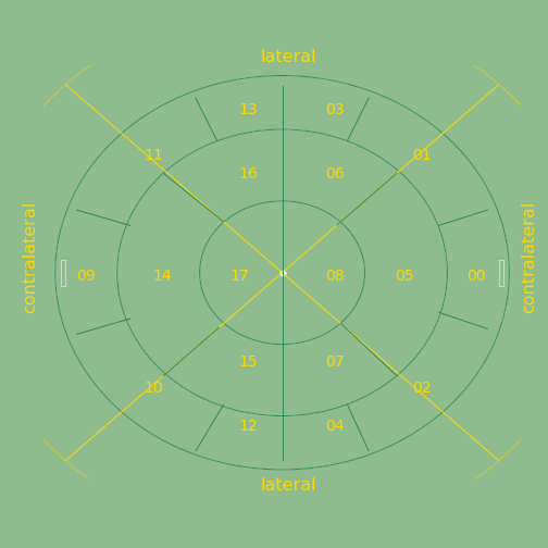
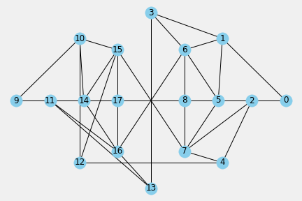
The aPLandscape is shown in Figure 1.2.1. and modeled as the network graph PL in Figure 1.2.2.

#collapse_hide
# aNT's Patch proposal for the Inside Patched Landscape in aFootball
PL = nx.Graph(name='PL-aFootball')

#, patch='a', lane='central', zone='z1', half='us', poss=0,
#             patch_org={0,0}, patch_max={100,100}, bip={'x':50,'y':50})
#it is a eighteen_patch_zones_graph indeed

PL.add_node( 0, patch='00',pwU='inside',half='own',subsp='box')
#,zone='z1',poss=0, patch_org=(xmin,ymin),patch_max=(boxEdgeus,boxEdgeLeft),bip={'x':xcb,'y':ycb})
PL.add_node( 1, patch='01',pwU='inside',half='own',subsp='outter')
#,zone='z1',poss=0,patch_org=(xmin,boxEdgeRight),patch_max=(boxEdgeus,ymax), bip={'x':xcc,'y':ycc})
PL.add_node( 2, patch='02',pwU='inside',half='own',subsp='outter')
#,zone='z1',poss=0, patch_org=(boxEdgeus,boxEdgeLeft + gl3),patch_max=(halfwayline,boxEdgeRight - gl3),bip={'x':xcd,'y':ycd})
PL.add_node( 3, patch='03',pwU='inside',half='own',subsp='outter')
#,zone='z1',poss=0, patch_org=(boxEdgeus,boxEdgeLeft),patch_max=(halfwayline,boxEdgeLeft + gl3),bip={'x':xcf,'y':ycf})
PL.add_node( 4, patch='04',pwU='inside',half='own',subsp='outter')
#,zone='z1',poss=0, patch_org=(boxEdgeus,boxEdgeRight - gl3),patch_max=(halfwayline,boxEdgeRight),bip= {'x':xcg,'y':ycg})

PL.add_node( 5, patch='05',pwU='inside', half='own',subsp='inner')
#,zone='z1',poss=0, patch_org=(boxEdgeus,0),patch_max=(boxEdgeus + bl2us,boxEdgeLeft),bip={'x':xch,'y':ych})
PL.add_node( 6, patch='06',pwU='inside',half='own',subsp='inner')
#,zone='z1',poss=0, patch_org=(boxEdgeus,boxEdgeRight),patch_max=(boxEdgeus + bl2us,ymax), bip={'x':xcj,'y':ycj})
PL.add_node( 7, patch='07',pwU='inside',half='own',subsp='inner')
#,zone='z2',poss=0, patch_org=(boxEdgeus + bl2us,ymin),patch_max=(halfwayline,boxEdgeLeft), bip={'x':xck,'y':yck})
PL.add_node( 8, patch='08',pwU='inside',half='own',subsp='core')
#,zone='z2',poss=0, patch_org=(boxEdgeus + bl2us,boxEdgeRight),patch_max=(halfwayline,ymax), bip={'x':xcl,'y':ycl})

PL.add_node( 9, patch='09',pwU='inside',half='them',subsp='box')
#, zone='z2',poss=0, patch_org=(halfwayline,boxEdgeLeft),patch_max=(boxEdgeop,boxEdgeLeft + gl3),bip={'x':xcn,'y':ycn})
PL.add_node(10, patch='10',pwU='inside',half='them',subsp='outter')
#,zone='z2',poss=0, patch_org=(halfwayline,boxEdgeRight - gl3),patch_max=(boxEdgeop,boxEdgeRight),bip={'x':xcp,'y':ycp})
PL.add_node(11, patch='11',pwU='inside',half='them',subsp='outter')
#,zone='z2',poss=0, patch_org=(halfwayline,xmin),patch_max=(halfwayline + bl2op,boxEdgeLeft),bip={'x':xcq,'y':ycq})
PL.add_node(12, patch='12',pwU='inside',half='them',subsp='outter')
#,zone='z2',poss=0, patch_org=(halfwayline,boxEdgeRight),patch_max=(halfwayline + bl2op,ymax),bip={'x':xcr,'y':ycr})
PL.add_node(13, patch='13',pwU='inside',half='them',subsp='outter')
#,zone='z3',poss=0, patch_org=(halfwayline + bl2op,ymin),patch_max=(boxEdgeop,boxEdgeLeft),bip={'x':xcs, 'y':ycs})

PL.add_node(14, patch='14',pwU='inside',half='them',subsp='inner')
#,zone='z3',poss=0, patch_org=(halfwayline + bl2op,boxEdgeRight),patch_max=(boxEdgeop,ymax),bip={'x':xct,'y':yct})
PL.add_node(15, patch='15',pwU='inside',half='them',subsp='inner')
#,zone='z3',poss=0, patch_org=(boxEdgeop,ymin),patch_max=(xmax,boxEdgeLeft),bip={'x':xcv,'y':ycv})
PL.add_node(16, patch='16',pwU='inside',half='them',subsp='inner')
#,zone='z3',poss=0, patch_org=(boxEdgeop,boxEdgeRight),patch_max=(ymax,xmax),bip={'x':xcw,'y':ycw})

PL.add_node(17, patch='17',pwU='inside',half='them',subsp='core')
#, zone='z3',poss=0, patch_org=(boxEdgeop,boxEdgeLeft),patch_max=(xmax,boxEdgeLeft + gl3),bip={'x':xcx,'y':ycx})

#p = CircosPlot(PL, node_labels=True) #, node_color='pwU', node_grouping='pwU')
#p.draw()
#plt.savefig("../../APimages/aPLandscape_whole_aFootball")
#plt.show()
#collapse_hide
PL.add_edge(0,0)
PL.add_edge(0,1)
PL.add_edge(0,2)
PL.add_edge(0,5)

PL.add_edge(1,1)
PL.add_edge(1,0)
PL.add_edge(1,3)
PL.add_edge(1,5)
PL.add_edge(1,6)

PL.add_edge(2,2)
PL.add_edge(2,0)
PL.add_edge(2,4)
PL.add_edge(2,5)
PL.add_edge(2,7)

PL.add_edge(3,3)
PL.add_edge(3,1)
PL.add_edge(3,6)
PL.add_edge(3,13)

PL.add_edge(4,4)
PL.add_edge(4,2)
PL.add_edge(4,7)
PL.add_edge(4,12)

PL.add_edge(5,5)
PL.add_edge(5,0)
PL.add_edge(5,1)
PL.add_edge(5,2)
PL.add_edge(5,6)
PL.add_edge(5,7)
PL.add_edge(5,8)

PL.add_edge(6,6)
PL.add_edge(6,1)
PL.add_edge(6,3)
PL.add_edge(6,5)
PL.add_edge(6,8)
PL.add_edge(6,16)

PL.add_edge(7,7)
PL.add_edge(7,2)
PL.add_edge(7,4)
PL.add_edge(7,5)
PL.add_edge(7,8)
PL.add_edge(7,15)

PL.add_edge(8,8)
PL.add_edge(8,5)
PL.add_edge(8,6)
PL.add_edge(8,7)
PL.add_edge(8,17)

PL.add_edge(9,9)
PL.add_edge(9,10)
PL.add_edge(9,11)
PL.add_edge(9,14)

PL.add_edge(10,10)
PL.add_edge(10,9)
PL.add_edge(10,12)
PL.add_edge(10,14)
PL.add_edge(10,15)

PL.add_edge(11,11)
PL.add_edge(11,9)
PL.add_edge(11,13)
PL.add_edge(11,14)
PL.add_edge(11,16)

PL.add_edge(12,12)
PL.add_edge(12,4)
PL.add_edge(12,10)
PL.add_edge(12,15)

PL.add_edge(13,13)
PL.add_edge(13,3)
PL.add_edge(13,11)
PL.add_edge(13,16)

PL.add_edge(14,14)
PL.add_edge(14,9)
PL.add_edge(14,10)
PL.add_edge(14,11)
PL.add_edge(14,15)
PL.add_edge(14,16)
PL.add_edge(14,17)

PL.add_edge(15,15)
PL.add_edge(15,7)
PL.add_edge(15,10)
PL.add_edge(15,12)
PL.add_edge(15,14)
PL.add_edge(15,17)

PL.add_edge(16,16)
PL.add_edge(16,6)
PL.add_edge(16,11)
PL.add_edge(16,13)
PL.add_edge(16,14)
PL.add_edge(16,17)

PL.add_edge(17,17)
PL.add_edge(17,8)
PL.add_edge(17,14)
PL.add_edge(17,15)
PL.add_edge(17,16)
#collapse_hide
print("aPB-Football Universe: ")
print("      There is just the inside %d patches in the aPLandscape " % (PL.number_of_nodes()))
print("      and %d possible inter-patched zone interactions" % (PL.number_of_edges()))
print("      just the interior of aPLandscape with {core,inner,outter,box} 2D-subspaces")

p = CircosPlot(PL, node_labels=True, node_color='subsp')
p.draw()
#plt.savefig("../../APimages/Circos_aBlandscape_neighborhood")
The organization of space into meso subspaces sets reveals the existence of a terrain hierarchy of affordances in the aPLandscape that invites to respond with plays and tasks proper of an organismic aFootball style and strategy. One in which a core-assemble is a positional set up in order to create intermediate plays in the inner subspace and with a larger membrane-assemble positional set up where to execute transport tasks and mantain intermediate plays.
An n-players, where 1<n<=11, team can be positioned in a kind of convex closure or a shape that contains all outter patches. It is the convex hull, a geometric concept that emerges from the space architecture as a kind of complexity of the landscape. An invitation to move and play the ball in this convex hull that currently separates inner and outter subspaces and, defines a subsumed core subspace.
#collapse_hide
# Network Properties of PL graph
# Football aPLandscape with 3 Lane Interconnections
r = dict(nx.degree(PL))
nx.draw(PL, nodelist=r.keys(), with_labels=True, node_color='skyblue', node_size=[v*50 for v in r.values()], cmap=plt.cm.Blues)

#plt.savefig("inaFootball aPLandscape's Ball Flow")
plt.show()
#collapse_hide

# Tableau of Distances Between Patches in aPLandscape

pathlengths = []
#print("average shortest path length %s" % (sum(pathlengths) / len(pathlengths)))

print("source_pz (target_pz:length, )")
for z in PL.nodes():
    spl = dict(nx.single_source_shortest_path_length(PL, z))
    print('{} ({} '.format(z, spl))
    for p in spl:
        pathlengths.append(spl[p])

print("average shortest path length %s" % (sum(pathlengths)/len(pathlengths)))

#histogram of path legths
dist = {}
for p in pathlengths:
    if p in dist:
        dist[p] += 1
    else:
        dist[p] = 1

print("length #paths")
verts = dist.keys()
for d in sorted(verts):
    print('%s %d' % (d, dist[d]))


print("radius: %d" % nx.radius(PL))
print("diameter: %d" % nx.diameter(PL))
print("eccentricity: %s" % sorted(nx.eccentricity(PL)))
print("center: %s" % nx.center(PL))
print("periphery: %s" % nx.periphery(PL))
print("density: %s" % nx.density(PL))
| length | paths |
|---|---|
| 0 | 18 |
| 1 | 74 |
| 2 | 104 |
| 3 | 86 |
| 4 | 36 |
| 5 | 6 |
| pz | (target_pz:length, ) | Z |
|---|---|---|
| 0 | ({ 0:0, 1:1, 2:1, 5:1, 3:2, 6:2, 4:2, 7:2, 8:2,13:3,16:3,12:3,15:3,17:3,11:4,14:4,10:4, 9:5} | 45 |
| 1 | ({ 1:0, 0:1, 3:1, 5:1, 6:1, 2:2,13:2, 7:2, 8:2,16:2, 4:3,11:3,15:3,17:3,14:3,12:4, 9:4,10:4} | 41 |
| 2 | ({ 2:0, 0:1, 4:1, 5:1, 7:1, 1:2,12:2, 6:2, 8:2,15:2, 3:3,10:3,16:3,17:3,14:3,13:4, 9:4,11:4} | 41 |
| 3 | ({ 3:0, 1:1, 6:1,13:1, 0:2, 5:2, 8:2,16:2,11:2, 2:3, 7:3,17:3,14:3, 9:3, 4:4,15:4,10:4,12:5} | 45 |
| 4 | ({ 4:0, 2:1, 7:1,12:1, 0:2, 5:2, 8:2,15:2,10:2, 1:3, 6:3,17:3,14:3, 9:3, 3:4,16:4,11:4,13:5} | 45 |
| 5 | ({ 5:0, 0:1, 1:1, 2:1, 6:1, 7:1, 8:1, 3:2, 4:2,16:2,15:2,17:2,13:3,12:3,11:3,14:3,10:3, 9:4} | 35 |
| 6 | ({ 6:0, 1:1, 3:1, 5:1, 8:1,16:1, 0:2,13:2, 2:2, 7:2,17:2,11:2,14:2, 4:3,15:3, 9:3,10:3,12:4} | 35 |
| 7 | ({ 7:0, 2:1, 4:1, 5:1, 8:1,15:1, 0:2,12:2, 1:2, 6:2,17:2,10:2,14:2, 3:3,16:3, 9:3,11:3,13:4} | 35 |
| 8 | ({ 8:0, 5:1, 6:1, 7:1,17:1, 0:2, 1:2, 2:2, 3:2,16:2, 4:2,15:2,14:2,13:3,11:3,12:3,10:3, 9:3} | 35 |
| 9 | ({ 9:0,10:1,11:1,14:1,12:2,15:2,13:2,16:2,17:2, 4:3, 7:3, 3:3, 6:3, 8:3, 2:4, 5:4, 1:4, 0:5} | 45 |
| 10 | ({10:0, 9:1,12:1,14:1,15:1,11:2, 4:2,16:2,17:2, 7:2,13:3, 2:3, 6:3, 8:3, 5:3, 3:4, 0:4, 1:4} | 41 |
| 11 | ({11:0, 9:1,13:1,14:1,16:1,10:2, 3:2,15:2,17:2, 6:2,12:3, 1:3, 7:3, 8:3, 5:3, 4:4, 0:4, 2:4} | 41 |
| 12 | ({12:0, 4:1,10:1,15:1, 2:2, 7:2, 9:2,14:2,17:2, 0:3, 5:3, 8:3,11:3,16:3, 1:4, 6:4,13:4, 3:5} | 45 |
| 13 | ({13:0, 3:1,11:1,16:1, 1:2, 6:2, 9:2,14:2,17:2, 0:3, 5:3, 8:3,10:3,15:3, 2:4, 7:4,12:4, 4:5} | 45 |
| 14 | ({14:0, 9:1,10:1,11:1,15:1,16:1,17:1,12:2,13:2, 7:2, 6:2, 8:2, 4:3, 3:3, 2:3, 5:3, 1:3, 0:4} | 35 |
| 15 | ({15:0, 7:1,10:1,12:1,14:1,17:1, 2:2, 4:2, 5:2, 8:2, 9:2,11:2,16:2, 0:3, 1:3, 6:3,13:3, 3:4} | 35 |
| 16 | ({16:0, 6:1,11:1,13:1,14:1,17:1, 1:2, 3:2, 5:2, 8:2, 9:2,10:2,15:2, 0:3, 2:3, 7:3,12:3, 4:4} | 35 |
| 17 | ({17:0, 8:1,14:1,15:1,16:1, 5:2, 6:2, 7:2, 9:2,10:2,11:2,12:2,13:2, 0:3, 1:3, 2:3, 3:3, 4:3} | 35 |
| property | |
|---|---|
| av_path_length | 2.2037037 |
| radius | 3 |
| diameter | 5 |
| eccentricity | [0, 1, 2, 3, 4, 5, 6, 7, 8, 9, 10, 11, 12, 13, 14, 15, 16, 17] |
| center | [8, 17] |
| periphery | [0, 3, 4, 9, 12, 13] |
| density | 0.35947712418300654 |
The network properties of PL graph, the relational model of the aPLandscape’s interior, shows 18 nodes representing patches and 324 interactions of i-adjacency length, where i in {0,1,2,3,4,5} range. The total length of those interactions is 714 and an average shortest path length 2.20 patches.
Assume Mon, a second man, enters to the aPLandscape to constitute a minimal AcEmFC team {Gon, Mon}. Now on, there are 1132 possible Gon’s possible moves|passes of the ball from the centroid of each patch to the centroid of other patch, stasis included in the interior of the aPLandscape. To use these abundant set of affordances as opportunities to play; the minimal football team must adopt a positional football style.
The PL graph has small-world network properties: a combination of high local clustering of connections between topologically neighboring patches (178-out-of-324) that is associated with high topological efficiency of ball flow and short topological path lengths between any pair of patches (apl = 2.20). This is the reason to play in the aPLandscape a possessional football.
The high efficiency of ball flow in the aPLandscape can be achieved by using the relatively medium connection density (~36% of maximum - diameter=5 - inter-patch connectivity) that means must intermix local short ball translation with often global patch connectivity offered by 4-length paths or once-in-a-while with 5-length passes. Therefore, this style for trajectory creation must remember the ideas of progress to the opponent goal patch and the use of contralateral traslations in the end-up subphase that ends in the omega-point. One point to re-mark about the aPLandscape is the variable decreasing value of the parallel cords when approaching a goal thing2.
A network with a rich club property is identified if the set of nodes in the centre core [8,17] or inner [5,6,7,14,15,16] subspaces have high degree and are densely intra-connected. The set of nodes in the core-centre have low betwenness centrality in the same order of peripheral nodes. But, the set of nodes in the inner-centre have high betweenness centrality contribution and degrees (8,7,7) greater than of the set of nodes in the periphery of PL, as shown in Figure 1.2.4. Therefore, we claim the aPLandscape graph exhibit a rich club property associated to its most important set of inner-centre patches. This set of patches is the persistent objective of space-control during all the match duration.
| node | bc_contrib | degree | node | bc_contrib | degree | node | bc_contrib | degree |
|---|---|---|---|---|---|---|---|---|
| 0 | 0.01425 | 5 | 1 | 0.05561 | 6 | 2 | 0.05561 | 6 |
| 3 | 0.04527 | 5 | 4 | 0.04527 | 5 | 5 | 0.14973 | 8 |
| 6 | 0.15762 | 7 | 7 | 0.15762 | 7 | 8 | 0.06900 | 6 |
| 9 | 0.01425 | 5 | 10 | 0.05561 | 6 | 11 | 0.05561 | 6 |
| 12 | 0.04527 | 5 | 13 | 0.04527 | 5 | 14 | 0.14973 | 8 |
| 15 | 0.15762 | 7 | 16 | 0.15762 | 7 | 17 | 0.06900 | 6 |
#collapse_hide

import collections

degree_sequence = sorted([z for n, z in PL.degree()], reverse=True)
# print "Degree sequence". degree_sequence
degreeCount = collections.Counter(degree_sequence)
deg, cnt = zip(*degreeCount.items())
fig, ax = plt.subplots(figsize=(8,8))

plt.bar(deg, cnt,width=0.80, color='skyblue')
plt.suptitle("Degree Histogram of Patches in aPLandscape")
plt.ylabel("Count")
plt.xlabel("Degree")
ax.set_xticks([d + 0.4 for d in deg])
ax.set_xticklabels(deg)

#draw graph in inset
plt.axes([0.4, 0.4, 0.5, 0.5])
PLcc = sorted(nx.connected_component_subgraphs(PL), key=len, reverse=True)[0]
pos = nx.spring_layout(PLcc)
plt.axis('on')
nx.draw_networkx_nodes(PLcc, pos, with_labels=True, node_size=30, node_color=range(18), cmap=plt.cm.Blues)
nx.draw_networkx_edges(PLcc, pos, alpha=0.5)
#plt.savefig("../../APimages/DegreeHistogramPatchesinaPLandscape")
plt.show()
Other organization of the interior subscape in aPLandscape identifies an adjacency mesh between patches in which emerge {own-box, inner, outter, opponent-box} meso subspaces whose static structure is clearly identificable.

Another organization of the interior subspace in aPLandscape identifies other adjacency mesh between patches of meso subspaces {Own, Them, Both} that divides the landscape in own field and their field and the complete field can be seen as a both teams subspace.

Today, one main problem of the football analytical community ask how to value the distint zones of a football field taking into account its control importance for the expected goal possibility. Figure 1.2.7. shown an intrinsic tentative score goal value of each patch in function of its degree or number of adjacent patches and distance to the center of the opponent goal.

This information capture the importance of patches as team and players affordances for global and local ‘aPLandscape control’ [BarcaInnoHub-2020] estimates that current tracking systems operate at a rate of 25Hz and the event’s match dynamics generate an average of 2700 frames by half times. With our importance weight of the inner patches {5,6,7,14,15,16,8,17} subset patch’s centroids are reference points to explore as potential affordances of open space to be controlled for core synergons and the convex hull frontier between inner an outter subsets structures for membrane synergons.
The collective and individual effort of team and player has to be keep on-ball control, progress, inside the opponent half aPLandscape, to the opponent goal and try to end-up the trajectory structure construction as an effective Levy flight with a final ball action that scores a goal, and viceversa. In off-ball control, the motor task with respect to the value of patches subspaces is the inverse: Try to regain ball control, stop the progress of the opponents in our own half aPLandscape, the farest of our goal the better, and break or at least abort the risk of a conceded goal.
So, ball-control and patch subspaces-control are the key factors of our positional relations as a synergestic team during the match in order to evaluate our motor and strategic task efficiency. At the end, this efficiency has to correlate with the real one goal difference efficiency. Efficiency has to be the ratio between the number of own Levy flight built and intervals of simultaneous ball-control and opponent-subspace-control. So, the ratio between the number of opponent Levy flights built and the their interval of simultaneous ball-control and own-subspace-control.
Any bounded, patched territory is near (binary, ternary) decomposable [H.Simon-1978] into a hierarchical organization levels. This hierarchical space architecture of the aPLandscape can be build with a sequence of binary partitions.
- The "circular inside aPLandscape space" is partitioned into halves by a middle line l1 to separate {our-half, their-half}
- Each half subspace is partitioned by a semi-circle l2 line to distinguish {outter, inner} subspaces
- Each inner subspace inside a half subspace is partitioned by a semi-circle l3 line has to distinguish between (core, middle) subspaces
- The core-inner-half subspace identify a unique core patch {08} or {17}
- The middle-inner-half subspace must be ternary decomposable by means of a sequence of two partitions
- A right-lateral line l4 separate {left-inner, central.right-inner} in our-half and {right-inner, central.left-inner} in our-half. Therefore, patch {07}, as our left-inner subspace, and patch {16}, as their right-inner subspace, are uniquely identified.
- Each composed {central.right-inner} and {central.left-inner} subspaced are partitioned by the left-lateral line l5 to uniquely distinguish {central-inner, right-inner} subspaces in our half as {05} and {06} unique patches, and {central-inner, left-inner} subspaces in their half as {14} and {15} unique patches.
- Each outter subspace of a half subspace has to distinguish {left,left-box,box,right-box,right} subspaces as unique outter patches
- A 1/8-right-lateral line l6 isolates patch (13) in a partition {right-right-outter, rest1-outter} in their outter-half subspace and isolates patch {04} in the partition {left-left-outter, rest2-outter} in our outter-half subspace
- A 3/8-right-lateral line l7 isolates patch {11} in their rest1-outter subspace and isolates patch {02} in our rest1-outter subspace in the partition {right-center-outter, rest2-outter}
- A 5/8-left-lateral line l8 isolates patch {09} by partitioned the rest2-outter {their-box,rest3-outter} and isolate patch {00} by partioned our rest2-outter into {our-box, rest3-outter}
- A 7/8-left-lateral line l9 isolate patch {10} and {patch {12} by partioned their rest3-outter into {left-center-outter, left-left-outter} subspaces and isolate patch {01} and patch {03} by partitioned own rest3-outter into {right-center-outter,right-right-outter}
- Each inner subspace inside a half subspace is partitioned by a semi-circle l3 line has to distinguish between (core, middle) subspaces
- Each half subspace is partitioned by a semi-circle l2 line to distinguish {outter, inner} subspaces
The multi-level hierarchy of relevant subspaces of the aPLandscape constitute a BPS binary partition subspaces tree as reference catalog of the playground.
1. The perimeter lane and the goal lfixed locations on the aPBLandscape impose a global regulatory constrain on actual football flow by reducing degrees of freedom of Gon autonomy about which direction of play to choose next.↩
2. The reduced open subspaces as the ball is near to a goal is a first reason football is not played in a circular field with rotational symmetry↩