Interior Space Architecture in aPLandscape for Organic aFootball
Charles R Paez Monzon - 2020 - aNatureTechnologies
- ” …after all, on the pitch what we see are plays, not data” - Clement Lengled
- ” There is no exterior, just interior in the closed aFICS Football Universe and it is full of affordances” - aFICS Vision
- ” The main affordance of interior space architecture invites to play in an organic aFootball style” - aFICS Vision
- 5.1. Affordances, Landscape Fitness and aFICS Literacy
- 5.2. Graph Model of the Interior of the Patched Landscape
- 5.3. Affordance of Organic aFootball: Core-Convex_Hull Subspace Control
- 5.4. Network Properties of Space Architecture of aPLandscape
- Table 5.1. Number of Paths of i-adjacency length in the interior of aPLandscape
- Table 5.2. i-adjacency length of all possible single source patch-to-patch interactions in the interior of aPLandscape
- Table 5.3. Set of Network Properties of PL Graph Model of the Interior of aPLandscape
- Table 5.4. Betweenness Centrality Contribution of each Patch
- 5.4.1 Organization of Space in Meso Subspaces Sets
- 5.4.2. Value of Patch Subspaces Control
5.1. Affordances, Landscape Fitness and aFICS Literacy
Gon is learning to explore and exploit the PB_landscape. He is instructed to perceive the environment in behavioral terms. The set of things (goals, patch-zones, the ball) provides oportunities for agency to move or play, or affordances in order to answer the great question: What is to play football? that only depends of his own aFICS skills and his football action capabilities.
Affordances are properties of the coupled dynamical systems Gon-PB_Landscape, scaled to his action capabilities (strength, speed, reaction times, height, weight, body dimensions) and, affordances are perceived by Gon as he learn to establish a Gon-PB_Landscape fit.
Academia Emeritense knows that its first cognitive task in Gon’s aFICS footbal education is help him to acquiere the idea of perceive the patched landscape, and later the pitch, in relation to its functionality. Its meaning is in the affordances that provide insights in what Gon learns and how he accomplished the motor task with open inteligence that guides the decision making process of how and when to act.
Gon and AcEmFC know that learning a skill must be understood as the emergence of an adaptive, functional dynamic and constrained relation between he and his football environment fitness. This fit is influenced by a set of constrains, always present, due to
- His individual biophysical, emotional, mental and psycological constrains and,
- Environmental physical, patch-inherents constrains and most important its set of affordances offered to him in any event
All of them must be used and exploited by Gon as opportunities for his agency in the PB_Landscape and his actions will be observed by the head coach HC as a metric of his basic aFICS literacy.
In this perspective, Gon involves understanding of his whole body - embodied - with affordances offered by the - embedded - PB_landscape will determine his agency or task performance in the ground play. aFICS literacy is the metric used during his aFICS synergon development process until he left Academia Emeritense FC. Literacy must be understood by our talents as ‘being educated’ in our aFICS vision in the language game in the community.
Moreover, the perception of affordances evolves and changes as capability for skilled action improves. It is our responsability to offer, in the physical plant of our institution, through deliberate design facilities for enhance motor skills improvement.
Let me help any player an aid that expand his vision of the invisible that Clement Lengled does not consider… after all, on the PB_landscape we see affordances and plays, not data.
5.2. Graph Model of the Interior of the Patched Landscape
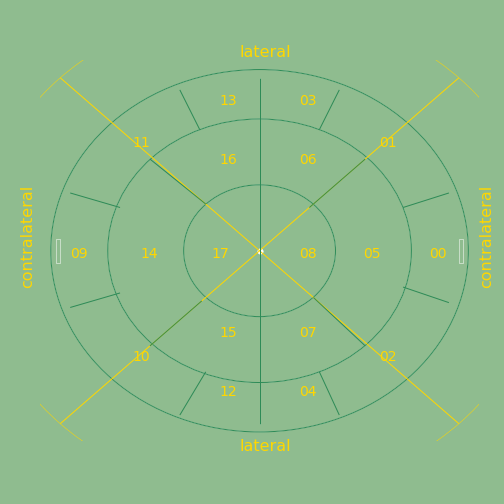
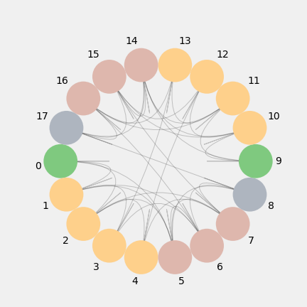
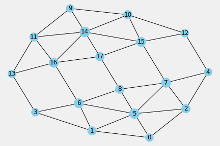
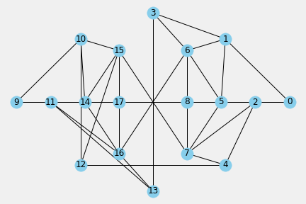
Let us move from the bounded landscape model of the aFootball Universe with a perimeter and an interior space to a more strict idea of an empty patched landscape without perimeter and just constitued for interior space. This landscape called aPLandscape has eighteen patch-zones {0,1,2,3,4,5,6,7,8,9,10,11,12,13,14,15,16,17} and fifty five bidirectional spatial- adjacency relationships between patches, included 18 spatial-adjecency self-relations of the patches themselves. The aPLandscape is shown in Figure 5.1. and modeled as the network graph PL in Figure 5.2.
5.3. Affordance of Organic aFootball: Core-Convex_Hull Subspace Control
The organization of space into meso subspaces sets reveals the existence of a terrain hierarchy of affordances in the aPLandscape that invites to responds with plays and tasks propers of an organic aFootball style and strategy. One in which a core-modulus is a positional set up in order to plays in the inner subspace and with a larger membrane-modulus positional set up. One possisioned in a kind of convex closure of a shape that contains all outter patches. It is the convex hull, a geometric concept that emerges from the space architecture as a kind of complexity of the landscape. An invitation to move and play the ball in this convex hull that currently separates inner and outter subspaces and, with a subsumed core modulus.
5.4. Network Properties of Space Architecture of aPLandscape
The network properties of PL graph, the relational model of the aPLandscape’s interior, shows 18 nodes representing patches and 324 interactions of i-adjacency length, where i in {0,1,2,3,4,5} range. The total length of those interactions is 714 and an average shortest path length 2.2037037
There are 1132 possible Gon’s moves|passes of the ball from the centroid of each patch to the centroid of other patch, stasis included in the interior of the aPLandscape. To use these abundant affordances as opportunities to play the football team must be centered in possitional football style.
The PL graph has small-world network properties: a combination of high local clustering of connections between topologically neighboring patches (178-out-of-324) that is associated with high topological efficiency of ball flow and short topological path lengths between any pair of patches (apl = 2.20). This is the reason to play in the aPLandscape a possessional football
The high efficiency of ball flow in the aPLandscape can be achieved by using the relatively medium connection density (~36% of maximum - diameter=5 - inter-patch connectivity) that means must intermix local short ball translation with often global patch connectivity offered by 4-length paths or once-in-a-while with 5-length passes. Therefore, this style of trajectory creation must remember the ideas of progress to the opponent goal patch and the use of contralateral traslations in the end- up subphase that ends in the omega-point. One point to re-mark about the aPLandscape is the variable decreasing value of the parallel cords when approaching a goal thing.
Table 5.1. Number of Paths of i-adjacency length in the interior of aPLandscape
| length | #paths |
|---|---|
| 0 | 18 |
| 1 | 74 |
| 2 | 104 |
| 3 | 86 |
| 4 | 36 |
| 5 | 6 |
Table 5.2. i-adjacency length of all possible single source patch-to-patch interactions in the interior of aPLandscape
| pz | (target_pz:length, ) | Z |
|---|---|---|
| 0 | ({0: 0, 1: 1, 2: 1, 5: 1, 3: 2, 6: 2, 4: 2, 7: 2, 8: 2, 13: 3, 16: 3, 12: 3, 15: 3, 17: 3, 11: 4, 14: 4, 10: 4, 9: 5} | 45 |
| 1 | ({1: 0, 0: 1, 3: 1, 5: 1, 6: 1, 2: 2, 13: 2, 7: 2, 8: 2, 16: 2, 4: 3, 11: 3, 15: 3, 17: 3, 14: 3, 12: 4, 9: 4, 10: 4} | 41 |
| 2 | ({2: 0, 0: 1, 4: 1, 5: 1, 7: 1, 1: 2, 12: 2, 6: 2, 8: 2, 15: 2, 3: 3, 10: 3, 16: 3, 17: 3, 14: 3, 13: 4, 9: 4, 11: 4} | 41 |
| 3 | ({3: 0, 1: 1, 6: 1, 13: 1, 0: 2, 5: 2, 8: 2, 16: 2, 11: 2, 2: 3, 7: 3, 17: 3, 14: 3, 9: 3, 4: 4, 15: 4, 10: 4, 12: 5} | 45 |
| 4 | ({4: 0, 2: 1, 7: 1, 12: 1, 0: 2, 5: 2, 8: 2, 15: 2, 10: 2, 1: 3, 6: 3, 17: 3, 14: 3, 9: 3, 3: 4, 16: 4, 11: 4, 13: 5} | 45 |
| 5 | ({5: 0, 0: 1, 1: 1, 2: 1, 6: 1, 7: 1, 8: 1, 3: 2, 4: 2, 16: 2, 15: 2, 17: 2, 13: 3, 12: 3, 11: 3, 14: 3, 10: 3, 9: 4} | 35 |
| 6 | ({6: 0, 1: 1, 3: 1, 5: 1, 8: 1, 16: 1, 0: 2, 13: 2, 2: 2, 7: 2, 17: 2, 11: 2, 14: 2, 4: 3, 15: 3, 9: 3, 10: 3, 12: 4} | 35 |
| 7 | ({7: 0, 2: 1, 4: 1, 5: 1, 8: 1, 15: 1, 0: 2, 12: 2, 1: 2, 6: 2, 17: 2, 10: 2, 14: 2, 3: 3, 16: 3, 9: 3, 11: 3, 13: 4} | 35 |
| 8 | ({8: 0, 5: 1, 6: 1, 7: 1, 17: 1, 0: 2, 1: 2, 2: 2, 3: 2, 16: 2, 4: 2, 15: 2, 14: 2, 13: 3, 11: 3, 12: 3, 10: 3, 9: 3} | 35 |
| 9 | ({9: 0, 10: 1, 11: 1, 14: 1, 12: 2, 15: 2, 13: 2, 16: 2, 17: 2, 4: 3, 7: 3, 3: 3, 6: 3, 8: 3, 2: 4, 5: 4, 1: 4, 0: 5} | 45 |
| 10 | ({10: 0, 9: 1, 12: 1, 14: 1, 15: 1, 11: 2, 4: 2, 16: 2, 17: 2, 7: 2, 13: 3, 2: 3, 6: 3, 8: 3, 5: 3, 3: 4, 0: 4, 1: 4} | 41 |
| 11 | ({11: 0, 9: 1, 13: 1, 14: 1, 16: 1, 10: 2, 3: 2, 15: 2, 17: 2, 6: 2, 12: 3, 1: 3, 7: 3, 8: 3, 5: 3, 4: 4, 0: 4, 2: 4} | 41 |
| 12 | ({12: 0, 4: 1, 10: 1, 15: 1, 2: 2, 7: 2, 9: 2, 14: 2, 17: 2, 0: 3, 5: 3, 8: 3, 11: 3, 16: 3, 1: 4, 6: 4, 13: 4, 3: 5} | 45 |
| 13 | ({13: 0, 3: 1, 11: 1, 16: 1, 1: 2, 6: 2, 9: 2, 14: 2, 17: 2, 0: 3, 5: 3, 8: 3, 10: 3, 15: 3, 2: 4, 7: 4, 12: 4, 4: 5} | 45 |
| 14 | ({14: 0, 9: 1, 10: 1, 11: 1, 15: 1, 16: 1, 17: 1, 12: 2, 13: 2, 7: 2, 6: 2, 8: 2, 4: 3, 3: 3, 2: 3, 5: 3, 1: 3, 0: 4} | 35 |
| 15 | ({15: 0, 7: 1, 10: 1, 12: 1, 14: 1, 17: 1, 2: 2, 4: 2, 5: 2, 8: 2, 9: 2, 11: 2, 16: 2, 0: 3, 1: 3, 6: 3, 13: 3, 3: 4} | 35 |
| 16 | ({16: 0, 6: 1, 11: 1, 13: 1, 14: 1, 17: 1, 1: 2, 3: 2, 5: 2, 8: 2, 9: 2, 10: 2, 15: 2, 0: 3, 2: 3, 7: 3, 12: 3, 4: 4} | 35 |
| 17 | ({17: 0, 8: 1, 14: 1, 15: 1, 16: 1, 5: 2, 6: 2, 7: 2, 9: 2, 10: 2, 11: 2, 12: 2, 13: 2, 0: 3, 1: 3, 2: 3, 3: 3, 4: 3} | 35 |
Table 5.3. Set of Network Properties of PL Graph Model of the Interior of aPLandscape
| property | |
|---|---|
| av_path_length | 2.2037037 |
| radius | 3 |
| diameter | 5 |
| eccentricity | [0, 1, 2, 3, 4, 5, 6, 7, 8, 9, 10, 11, 12, 13, 14, 15, 16, 17] |
| center | [8, 17] |
| periphery | [0, 3, 4, 9, 12, 13] |
| density | 0.35947712418300654 |
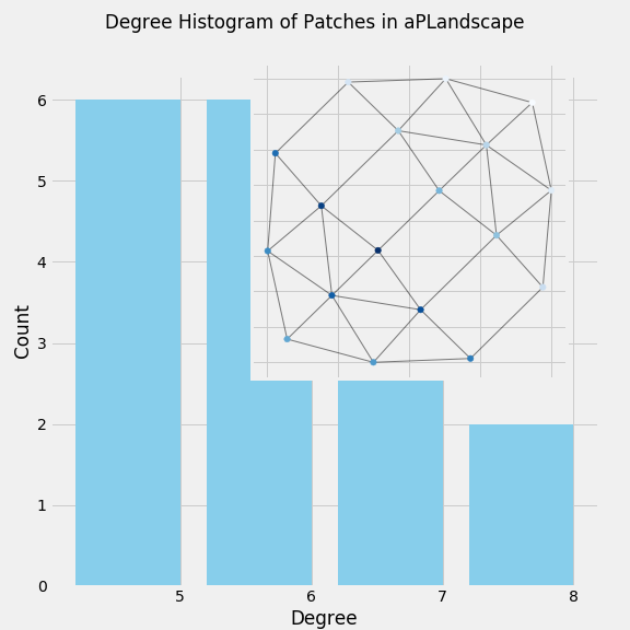
A network with a rich club property is identified if the set of nodes in the centre core [8,17] or inner [5,6,7,14,15,16] subspaces have high degree and are densely intra-connected. The set of nodes in the core-centre have low betwenness centrality in the same order of peripheral nodes. But, the set of nodes in the inner-centre have high betweenness centrality contribution and degrees (8,7,7) greater than of the set of nodes in the periphery of PL, as shown in Figure 5.4. Therefore, we claim the aPLandscape graph exhibit a rich club property associated to its most important set of inner-centre patches. This set of patches is the persistent objective of space-control during all the match duration.
Table 5.4. Betweenness Centrality Contribution of each Patch
| node | bc_contrib | degree | node | bc_contrib | degree | node | bc_contrib | degree |
|---|---|---|---|---|---|---|---|---|
| 0 | 0.01425 | 5 | 1 | 0.05561 | 6 | 2 | 0.05561 | 6 |
| 3 | 0.04527 | 5 | 4 | 0.04527 | 5 | 5 | 0.14973 | 8 |
| 6 | 0.15762 | 7 | 7 | 0.15762 | 7 | 8 | 0.06900 | 6 |
| 9 | 0.01425 | 5 | 10 | 0.05561 | 6 | 11 | 0.05561 | 6 |
| 12 | 0.04527 | 5 | 13 | 0.04527 | 5 | 14 | 0.14973 | 8 |
| 15 | 0.15762 | 7 | 16 | 0.15762 | 7 | 17 | 0.06900 | 6 |
5.4.1 Organization of Space in Meso Subspaces Sets
Other organization of the interior subscape in aPLandscape identifies an adjacency mesh between patches in which emerge {own- box, inner, outter, opponent box} meso subspaces whose structure is clearly identificable.
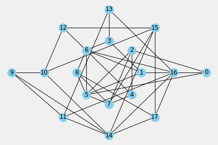
Another organization of the interior subspace in aPLandscape identifies other adjacency mesh between patches of meso subspaces {Own, Them, Both} that divides the landscape in own field and their field and the complete field can be seen as a both teams subspace.
5.4.2. Value of Patch Subspaces Control
Today, one main problem of the football analytical community ask how to value the distint zones of a football field taking into account its control importance for the expected goal possibility. Figure 5.7. shown an intrinsic score goal value of each patch in function of its degree or number of adjacent patches and distance to the center of the opponent goal.
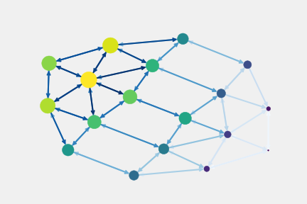
This information capture the importance of patches as team and players affordances for global and local ‘aPLandscape control’. [BarcaInnoHub] estimates that current tracking systems operate at a rate of 25Hz and the event’s match dynamics generate an average of 2700 frames by half times. With our importance weight of the inner patches {5,6,7,14,15,16,8,17} subset patches’ centroids are reference points to explore as potential affordances of open space to be controlled for core synergons and the ‘convex hull’ frontier between inner an outter subsets structures for membrane synergons. The collective and individual effort of team and player has to be keep on-ball control, progress, inside the opponent half aPLandscape, to the opponent goal and try to end-up the trajectory structure construction as an effective Levy flight with a final ball action that scores a goal, and viceversa. In off-ball control, the motor task with respect to the value of patches subspaces is the inverse: Try to regain ball control, stop the progress of the opponents in our own half aPLandscape, the farest of our goal the better, and break or at least abort the risk of a conceded goal.
So, ball-control and patch subspaces-control are the key factors of our possitional relations as a synergestic team during the match in order to evaluate our motor and strategic task efficiency. At the end, this efficiency has to correlate with the real one goal difference efficiency. Efficiency has to be the ratio between the number of own Levy flight built and intervals of simultaneous ball-control and opponent-subspace-control. So, the ratio between the number of opponent Levy flights built and the their interval of simultaneous ball-control and own-subspace-control.